Setting up a simple wind simulation with Phoenics

Content

To make a quick start possible a basic model with one high rise building is described. The building has a height of 200 m and a size of 50 x 50 m. The calculation domain has a size of l x b x h = 500 x 500 x 500 m. At the start there are no surrounding buildings. The terrain roughness is 3 m, which is representative for the centre of a large city. The wind speed is assumed to be 15 m/s at the reference height of 60 m, as shown in figure 5. The wind profile is assumed to be a power law with a power value of 0.36, as for a city centre.

Go to > file > start a new case, choose Flair

Fig. 1: Image when starting a new case

Enable the VR Viewer by > VIEW > Control Panel
Go to the VR Editor > Menu > Geometry > set the domain Size on x, y, z on 500 x 500 x 500 m and click OK.

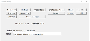
Fig. 2: First steps to make a domain geometry

Enable the Movement panel, by going to View > Movement control > Reset > fit to window > Apply > OK

Fig. 3: Making the large domain visible on the screen

Fig. 4: Creating a blockage and give it a location in the domain

Go to the VR Editor > Object > new > new object blockage
Give block1 the Name building1 and the Size 50 x 50 x 200 m
Locate building1 at the Object position x = 200 m and y = 200 m in Place
Click on Ok and close the Object management window.

You now have made your first Phoenics Model.

Fig. 5: The first input result

Remark: To see depth, go to Settings > Depth Effect and play with the slider. For the following please do not use the depth effect.

Click on the mesh toggle and an already refined grid is presented. The amount of cells is 39 x 39 x 34 = 51.714 cells, as can be seen from

Menu > Geometry in the row Number of cells.

Fig. 6: First result, without adaptation of the grid.

In order to know the wind velocity at a height of 1,75 the grid above the ground should be refined.

Click on the lowest section of the cells and adapt the values in z-direction as follows:

Fig. 7: Refined settings of the “Geometry” tab

Change the head of the z-direction in from Z-Auto to Z-Manual, increase the amount of cells from 16 to 45, use Distribution > Geom Prog and change symmetric in No (ignore the message), and change the power/ratio to 1.1. Close the Geometry windowSet the position of the red pencil on x, y, z = 255, 198, 1.75 m. in VR Editor > Position. The result is the following image:

Fig. 7: The highest density of the cells is close to the building in all directions

In order to know the wind velocity at a height of 1,75 the grid above the ground should be refined.

Click on the lowest section of the cells and adapt the values in z-direction as follows.

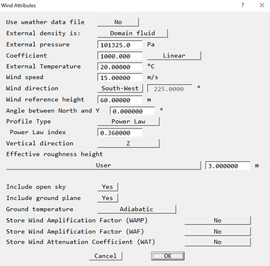
Fig. 8: Settings of the object “Wind”

Change in Objects > Wind > attributes the wind speed to 15 m/s, the reference height in 60 m, the wind direction in South-West. Choose for Profile Type > Power law and set the power law value on 0.36 (this is comparable with a city centre with high buildings). Set the Effective roughness height, after using “user” on 3 m and include this in the sky and the ground plane.
Close the Wind object.
Go to Menu > Gravitational forces > On
Go to Menu > Models > Turbulence models > KE Variants > RNG KE model.

Optional: Set in Numerics > Relaxation control > automatic convergence control > off and change the buttons of U1, V1 and W1 from LINEAR in FALSEDT (false time-step). Change the factors of U1, V1 and W1 from 1 to 0.1 (second). This is to reduce calculation time and increase accuracy as advised by the Phoenics helpdesk this year.

Set in Numerics the amount of Iterations to 500 and close the Menu window.
Save your Case via File > Save as a case. Give your file a name.
Go to Run > Solver and your first wind-simulation will start. A typical time needed to run this simulation is 6 minutes.

Fig. 9: Numerical presentation of the CFD-calculation and convergence process. “Values” is the physical parameter value at the location of the probe.

Table 1: Presentation and summary of the quality of the convergence, no errors are reported

> Making results visible

The following pictures can be made after the following steps.

Go to Run > postprocessor> VR Viewer. Use current result files. Click on “v” in the VR viewer to show the velocities. Click on the “contour”-toggle (box with red shape) to show contours of similar airflows and click on the arrow to show the direction arrows of the airflow.
Set the Probe position of the red pencil on x, y, z = 255, 198, 1.75 m again.
Make a picture perpendicular to the y-direction. Select the Y-direction, Y, in the VR viewer to display the contours and arrows in the Y plane. Select the Y view direction via select -Y through the Reset button in the main toolbar.
Make a similar picture of the contours and arrows in the Z-plane and show the information in the +Z direction.

Fig. 10: Cross-section, view from the South

Fig. 11: Horizontal section, wind from the South-West at a height of 1.75 m. The blue arrow is the North. The wind with the highest velocity is coming from the South-West which is presented with the red arrow.

The blue arrow is the North. The wind with the highest velocity is coming from the South-West, as given in the input, and is represented with the red arrow.

> Checking the Source Balance

It is very important to know whether the inflows and outflows of mass and energy are in balance. If they are, it is a good sign that the solution is convergent. If they are not, the solution is definitely not converged.

Open the Object Management dialog, and right-click on the Domain entry. From the context menu select 'Show nett sources'. This will display the sources and sinks of all variables.

The section showing 'Nett source of R1 at...' shows the mass source in kg/s at each inlet and outlet.

Fig. 12: Nett sources inlet and outlet flow.

Positive values are inflows,negative values are outflows. The 'nett sum' at the end of the section should be close to zero, as all the mass entering must leave. In this case, -8,95 kg/s is very small compared to the total flow in of 1.0076E+07 and the total outflow of 1.0076E+07. Based on the mass balance, the solution is converged.

> Wind nuisance analysis

> Quality of the design with respect to wind nuisance using 'Assessment of wind nuisance'

i. The wind pattern of the location at a height of 60 must be determined, following the calculation program from the NPR 6097.

From the weather data, a windspeed of 15 m/s at a height of 60 meters is taken as the input for the CFD program.
Chosen is a power law windprofile for a city centre with high buildings, i.e. an α of 0.36 and a gradient altitude of 500 m. The relevant values are then calculated as:

Average wind velocity at boundary height

Average wind speed at 1.75 m (walking)

Wind variation

Maximum wind velocity due to a gust at 1.75 meter (walking)

thus

ii. In a CFD program or wind tunnel the velocity at a height of 1.75 m above the ground for 12 wind directions and critical locations are determined. This velocity is related to a reference air velocity at a height of 60 m.

In this example only the South-West direction is determined, as this is the most important wind direction on this location.

The average wind speed at 1.75 m, according to the theory, is 4.2 m/s which is close to the average wind speed of 6.2 m/s calculated by Phoenics at a height 1.75 m, as can be seen on the upper right hand corner of the graph in the Z-direction. In the CFD-model the roughness of the city is very high which can explain the difference.

The hand calculated average wind velocity at boundary height (500 m) is 32.1 m/s. This value is close to the maximum velocity of 32 m/s in the CFD results, see the legend of figure 10.

The highest wind speeds are generally found near the corners of a building (Verhoeven, 1982). The velocity at the probe position at the height of 1.75 m near the corner of the building can be found in the upper right-hand corner of the CFD result and is 16.9 m/s. According to the table 2 in Assessment of wind nuisance, this is dangerous when strolling around the building.

Also, wind gusts can give problems (Verhoeven 1982). It is possible to assess the effect of wind-gusts under the assumption that the wind velocity is 15 m/s at a height of 60 m. The maximum wind velocity due to a gust at 1.75 meter (walking) was calculated to be 15.4 m/s, which is dangerous according to table 1 in Computational Domain.

iii. The amount of hours per year that a wind velocity of 5 m/s (wind comfort) or 15 m/s (wind danger) at the location is exceeded is assessed.

Comparing the simulated average wind speed of 2.6 with the simulated wind speed at the corner of the building, which is 9.0 m/s, the wind amplification factor (c) of this building can be calculated. The wind amplification value is the simulated wind speed at a certain position divided by the average wind speed at that height. In this case this value is 16.9/ 6.2 = 2.7, which could be expected as given by Verhoeven (1982).

Assuming a multiplication factor of 2.7, the windspeed at 60 m height should be no more than 15/2.7 = 5.5 m/s at 60 meter height. This happens more than 20 % of the time, according to figure 7 in Assessment of wind nuisance. The corners of this building are therefore Poor for Traversing, Stroling or Sitting.

There are around 30 hours that the windspeed at 60 m is above 15 m/s in figure 7. This is 30/6079 ~ 0.5 % of the time. At these 30 hours, the wind speed at pedestrian height (1.75 m) is 16.7 m/s, thus dangerous wind.

> Quality of the design with respect to wind speed

In this case the maximum velocity in the free field is 6.2 (from CFD) + 11.2 (calculated gust) = 17.4 m/s. At the corner of the simulated building this is more: 16.8 (from CFD) + 11.2 (calculated gust) = 28.0 m/s. The local wind speed can become 27.9 m/s and corresponds to category E of wind comfort. Figure 12 shows that at this wind speed it becomes difficult to keep your balance when walking. Entrances and walkways should therefore not be positioned at these corners or the design of the building should be altered to improve the wind comfort around the building. See for more design information the reader by Verhoeven (2018) and the other references given below.

Table 2: Wind comfort situations in daily life.

> How to improve the wind climate around the building

> Add a setback or a podium

According to the reader “Wind Nuisance” (Yoshie et al., 2007), a setback or a podium is a solution to improve the wind climate around the building. This was also done next to the very tall building on the TUDelft campus.

Fig. 13: Setback and podia around a high rise building (Yoshie R, Mochida A, Tominaga Y, Kataoka H, Harimoto K, Nozu T, Shirasawa T. Cooperative project for CFD prediction of pedestrian wind environment in the Architectural Institute of Japan. Journal of Wind Engineering and industrial Aerodynamics 95. 2007)

To show that it works, do the following:

Add a block of 80 m x 10 m x 5 meter on position 225 m x 195 m.
Change the head of the z-direction in from Z-Manual to Z-Auto again to change the grid.
Change the head of the z-direction in from Z-Auto to Z-Manual, increase the amount of cells as shown below.

Fig. 14: Grid settings small podium

Close the Geometry window. Set the position of the red pencil on x, y, z = 255, 190, 1.75 m. in VR Editor > Position.

After solving the solution, you now see that the average value is similar, but the air velocities close to the right-hand corner is lower, from 16.7 m/s to 12.1 m/s. Still not as low as you would like, but better.

Fig. 15: Results small podium

> Add a larger podium

Now try a larger podium.

Add a block of 100 m x 20 m x 10 meter on position 220 m x 180 m.

Fig. 16: Size and position of the larger podium

Change the head of the z-direction in from Z-Manual to Z-Auto again to change the grid.
Change the head of the z-direction in from Z-Auto to Z-Manual, increase the amount of cells as shown below.

Fig. 17: Grid settings for the larger podium

Set the position of the red pencil on x, y, z = 255, 175, 1.75 m. in VR Editor > Position.
After solving, the velocities are even lower in this situation.

Fig. 18: Results for the larger podium

> More accurate calculations

> Increase the domain size

To check if the domain size has an influence, the domain size is increased to 800 x 800 x500 m3.

Fig. 19: Results larger podium, larger domain.

Fig. 20: Convergence data at 500 iterations, large podium, larger domain

The results of 1000 iterations shows better convergence but no significant changes in the velocities in the z-direction at 1.75 m height.

Fig. 21: Convergence data at 1000 iterations, large podium, larger domain

Fig. 22: Results larger podium, larger domain, 1000 iterations

> How to import your own building

It is possible to import your own building via object building1.

Go back to the original input file with one building.
Go to Object Building1 > Shape > CAD file and you can import files with different extensions.
Position the building at x = 200 m, Y = 150 m.

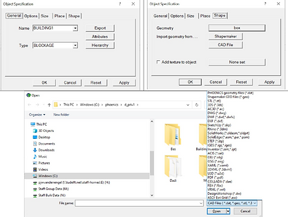
Fig. 23: Importing your own model

Fig. 24: Buttons to change the orientation of a shape in your object.

You can also add other blocks around your model.

In order to prevent an irregular grid (with only one cell beside a building) it is necessary than to recover the grid by making it “Automatic” for all the directions first. After that the z-direction can be put on “manual” again to increase the number of cells near the ground.

Remember to also put the probe at a different position, compared with the very simple building from 'How to make your first model?', for the solver and for the analysis.

You can find more tutorials about how to import your building in Phoenics in the Featured External Tutorials.