Some common non-linear kernels used for SVM include polynomial and radial basis function (RBF). You can find additional information about what kernels can be used on the SciKit Learn website

https://scikit-learn.org/stable/auto_examples/svm/plot_svm_kernels.html

Start by normalizing the data. To normalize data, it is best to use a pipeline because this first scales the training data and then applies the same scale to the test data without leading any training data.

# Import required functions

from sklearn.datasets import make_classification

from sklearn.linear_model import LogisticRegression

from sklearn.model_selection import train_test_split

from sklearn.pipeline import make_pipeline

from sklearn.preprocessing import StandardScaler

# Split dataset into training set and test set

X_train, X_test, y_train, y_test = train_test_split(wine.data, wine.target, test_size=0.3,random_state=109) # 70% training and 30% test

# Make pipeline for normalizing data

pipe = make_pipeline(StandardScaler(), LogisticRegression())

pipe.fit(X_train, y_train) # apply scaling on training data

pipe.score(X_test, y_test) # apply scaling on testing data, without leaking training data.

0.9259259259259259

Radial Basis Function (RBF) Kernel

SVM has a parameter called C which can be adjusted to allow for a certain level of mis-classification to have a more optimized location of the decision boundary.

When using the RBF kernel, there is another parameter, gamma, which can be adjusted to change how linear the boundary is.

From https://scikit-learn.org/stable/auto_examples/svm/plot_rbf_parameters.html:

"The gamma parameter defines how far the influence of a single training example reaches, with low values meaning ‘far’ and high values meaning ‘close’.

To find the best gamma and C values for RBF, it is a good idea to do an initial search. For this initial search, it is possible to use a logarithmic grid with basis 10.

from sklearn.svm import SVC

from sklearn.model_selection import StratifiedShuffleSplit

from sklearn.model_selection import GridSearchCV

C_range = np.logspace(-2, 10, 13)

gamma_range = np.logspace(-9, 3, 13)

param_grid = dict(gamma=gamma_range, C=C_range)

cv = StratifiedShuffleSplit(n_splits=5, test_size=0.2, random_state=42)

grid = GridSearchCV(SVC(), param_grid=param_grid, cv=cv)

grid.fit(X_train, y_train)

print("The best parameters are", grid.best_params_, "with a score of", grid.best_score_)

The best parameters are {'C': 100000.0, 'gamma': 1e-07} with a score of 0.944

Train the model based on the gamma and C values that were determined above.

#Import svm model

from sklearn import svm

#Create a svm Classifier

clf = svm.SVC(kernel="rbf", gamma=1e-07, C=100000.0) # RBF Kernel

#Train the model using the training sets

clf.fit(X_train, y_train)

#Predict the response for test dataset

y_pred = clf.predict(X_test)

#Import scikit-learn metrics module for accuracy calculation

from sklearn import metrics

# Model Accuracy: how often is the classifier correct?

print("Accuracy:",metrics.accuracy_score(y_test, y_pred))

# Which classes are commonly misclassified?

print('Confusion Matrix')

print(metrics.confusion_matrix(y_test, y_pred, labels=None))

Accuracy: 0.8703703703703703

Confusion Matrix

[[19 2 0]

[ 4 15 0]

[ 0 1 13]]

We can again visualize the decision boundary on the first 2 features of the dataset. It will take a few more seconds to run as it processes the data.

from sklearn.svm import SVC

import numpy as np

import matplotlib.pyplot as plt

from sklearn import svm, datasets

# Select 2 features / variable for the 2D plot that we are going to create.

X = wine.data[:, :2] # we only take the first two features.

y = wine.target

def make_meshgrid(x, y, h=.02):

x_min, x_max = x.min() - 1, x.max() + 1

y_min, y_max = y.min() - 1, y.max() + 1

xx, yy = np.meshgrid(np.arange(x_min, x_max, h), np.arange(y_min, y_max, h))

return xx, yy

def plot_contours(ax, clf, xx, yy, **params):

Z = clf.predict(np.c_[xx.ravel(), yy.ravel()])

Z = Z.reshape(xx.shape)

out = ax.contourf(xx, yy, Z, **params)

return out

model = svm.SVC(kernel='rbf', gamma=1e-07, C=100000.0)

clf = model.fit(X, y)

fig, ax = plt.subplots()

# create a mesh to plot in

h = .02 # step size in the mesh

x_min, x_max = X[:, 0].min() - 1, X[:, 0].max() + 1

y_min, y_max = X[:, 1].min() - 1, X[:, 1].max() + 1

xx, yy = np.meshgrid(np.arange(x_min, x_max, h),

np.arange(y_min, y_max, h))

Z = clf.predict(np.c_[xx.ravel(), yy.ravel()])

# Put the result into a color plot

Z = Z.reshape(xx.shape)

plt.contourf(xx, yy, Z, cmap=plt.cm.coolwarm, alpha=0.8)

# Plot also the training points

plt.scatter(X[:, 0], X[:, 1], c=y, cmap=plt.cm.coolwarm, edgecolors='k')

plt.xlabel('Alcohol')

plt.ylabel('Malic Acid')

plt.xlim(xx.min(), xx.max())

plt.ylim(yy.min(), yy.max())

plt.xticks(())

plt.yticks(())

plt.title("Decision Surface of SVM using RBF Kernel")

plt.show()

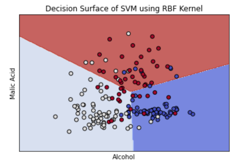
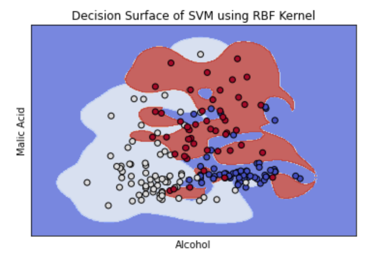
The graph above shows how the optimal parameters using the RBF kernel created an almost linear separation between the data. If we increase the gamma value, the separation boundary creates curves around specific groups of points. See this in the example below. For the sample dataset, this is less accurate. Additionally, higher gamma values can lead to overfitting.

from sklearn.svm import SVC import numpy as np import matplotlib.pyplot as plt from sklearn import svm, datasets # Select 2 features / variable for the 2D plot that we are going to create. X = wine.data[:, :2] # we only take the first two features. y = wine.target def make_meshgrid(x, y, h=.02): x_min, x_max = x.min() - 1, x.max() + 1 y_min, y_max = y.min() - 1, y.max() + 1 xx, yy = np.meshgrid(np.arange(x_min, x_max, h), np.arange(y_min, y_max, h)) return xx, yy def plot_contours(ax, clf, xx, yy, **params): Z = clf.predict(np.c_[xx.ravel(), yy.ravel()]) Z = Z.reshape(xx.shape) out = ax.contourf(xx, yy, Z, **params) return out model = svm.SVC(kernel='rbf', gamma=5, C=100000.0) clf = model.fit(X, y) fig, ax = plt.subplots()

# create a mesh to plot in h = .02 # step size in the mesh x_min, x_max = X[:, 0].min() - 1, X[:, 0].max() + 1 y_min, y_max = X[:, 1].min() - 1, X[:, 1].max() + 1 xx, yy = np.meshgrid(np.arange(x_min, x_max, h), np.arange(y_min, y_max, h)) Z = clf.predict(np.c_[xx.ravel(), yy.ravel()]) # Put the result into a color plot Z = Z.reshape(xx.shape) plt.contourf(xx, yy, Z, cmap=plt.cm.coolwarm, alpha=0.8) # Plot also the training points plt.scatter(X[:, 0], X[:, 1], c=y, cmap=plt.cm.coolwarm, edgecolors='k') plt.xlabel('Alcohol') plt.ylabel('Malic Acid') plt.xlim(xx.min(), xx.max()) plt.ylim(yy.min(), yy.max()) plt.xticks(()) plt.yticks(()) plt.title("Decision Surface of SVM using RBF Kernel") plt.show()

TASK: Plot a validation curve for the gamma value through SciKit Learn to see how the value of gamma impacts the accuracy of the model.

Polynomial kernel

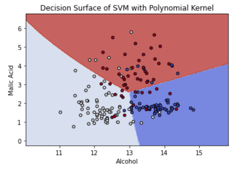
The polynomial kernel has three parameters: degree, gamma, and C. The most common degree used is either 2 or 3 because larger degrees are more likely to overfit. Gamma can be set to "auto" which means it uses 1 / n_features. C is the same as the C used for the RBF kernel.

#Import svm model

from sklearn import svm

#Create a svm Classifier

clf = svm.SVC(kernel="poly", degree=2, gamma="auto", C=100000.0) # Polynomial Kernel

#Train the model using the training sets

clf.fit(X_train, y_train)

#Predict the response for test dataset

y_pred = clf.predict(X_test)

#Import scikit-learn metrics module for accuracy calculation

from sklearn import metrics

# Model Accuracy: how often is the classifier correct?

print("Accuracy:",metrics.accuracy_score(y_test, y_pred))

# Which classes are commonly misclassified?

print('Confusion Matrix')

print(metrics.confusion_matrix(y_test, y_pred, labels=None))

Accuracy: 0.9259259259259259

Confusion Matrix

[[21 0 0]

[ 2 16 1]

[ 1 0 13]]

from sklearn.svm import SVC

import numpy as np

import matplotlib.pyplot as plt

from sklearn import svm, datasets

# Select 2 features / variable for the 2D plot that we are going to create.

X = wine.data[:, :2] # we only take the first two features.

y = wine.target

def make_meshgrid(x, y, h=.02):

x_min, x_max = x.min() - 1, x.max() + 1

y_min, y_max = y.min() - 1, y.max() + 1

xx, yy = np.meshgrid(np.arange(x_min, x_max, h), np.arange(y_min, y_max, h))

return xx, yy

def plot_contours(ax, clf, xx, yy, **params):

Z = clf.predict(np.c_[xx.ravel(), yy.ravel()])

Z = Z.reshape(xx.shape)

out = ax.contourf(xx, yy, Z, **params)

return out

model = svm.SVC(kernel='rbf')

clf = model.fit(X, y)

fig, ax = plt.subplots()

# Set-up grid for plotting.

X0, X1 = X[:, 0], X[:, 1]

xx, yy = make_meshgrid(X0, X1)

plot_contours(ax, clf, xx, yy, cmap=plt.cm.coolwarm, alpha=0.8)

ax.scatter(X0, X1, c=y, cmap=plt.cm.coolwarm, s=20, edgecolors='k')

ax.set_xlabel('Alcohol')

ax.set_ylabel('Malic Acid')

ax.set_title('Decision Surface of SVM with Polynomial Kernel')

plt.show()

TASK: Plot a validation curve for the degree value through SciKit Learn to see how the number of degrees impacts the accuracy of the model.