#Import scikit-learn dataset library

from sklearn import datasets

#Load dataset

wine = datasets.load_wine()

Print dataset information to understand the data.

# print the names of the features

print("Features: ", wine.feature_names)

# print the label classes

print("Labels: ", wine.target_names)

Features: ['alcohol', 'malic_acid', 'ash', 'alcalinity_of_ash', 'magnesium', 'total_phenols', 'flavanoids', 'nonflavanoid_phenols', 'proanthocyanins', 'color_intensity', 'hue', 'od280/od315_of_diluted_wines', 'proline']

Labels: ['class_0' 'class_1' 'class_2']

# print data(feature)shape

wine.data.shape

(178, 13)

# print the (top 5 records)

print(wine.data[0:5])

[[1.423e+01 1.710e+00 2.430e+00 1.560e+01 1.270e+02 2.800e+00 3.060e+00

2.800e-01 2.290e+00 5.640e+00 1.040e+00 3.920e+00 1.065e+03]

[1.320e+01 1.780e+00 2.140e+00 1.120e+01 1.000e+02 2.650e+00 2.760e+00

2.600e-01 1.280e+00 4.380e+00 1.050e+00 3.400e+00 1.050e+03]

[1.316e+01 2.360e+00 2.670e+00 1.860e+01 1.010e+02 2.800e+00 3.240e+00

3.000e-01 2.810e+00 5.680e+00 1.030e+00 3.170e+00 1.185e+03]

[1.437e+01 1.950e+00 2.500e+00 1.680e+01 1.130e+02 3.850e+00 3.490e+00

2.400e-01 2.180e+00 7.800e+00 8.600e-01 3.450e+00 1.480e+03]

[1.324e+01 2.590e+00 2.870e+00 2.100e+01 1.180e+02 2.800e+00 2.690e+00

3.900e-01 1.820e+00 4.320e+00 1.040e+00 2.930e+00 7.350e+02]]

# print the class labels

print(wine.target)

[0 0 0 0 0 0 0 0 0 0 0 0 0 0 0 0 0 0 0 0 0 0 0 0 0 0 0 0 0 0 0 0 0 0 0 0 0

0 0 0 0 0 0 0 0 0 0 0 0 0 0 0 0 0 0 0 0 0 0 1 1 1 1 1 1 1 1 1 1 1 1 1 1 1

1 1 1 1 1 1 1 1 1 1 1 1 1 1 1 1 1 1 1 1 1 1 1 1 1 1 1 1 1 1 1 1 1 1 1 1 1

1 1 1 1 1 1 1 1 1 1 1 1 1 1 1 1 1 1 1 2 2 2 2 2 2 2 2 2 2 2 2 2 2 2 2 2 2

2 2 2 2 2 2 2 2 2 2 2 2 2 2 2 2 2 2 2 2 2 2 2 2 2 2 2 2 2 2]

# Plot two of the features

import numpy as np

import matplotlib.pyplot as plt

# Plot the records here

data_0 = np.array([w[0] for w in zip(wine.data[:,[0,1]], wine.target) if w[1] == 0])

data_1 = np.array([w[0] for w in zip(wine.data[:,[0,1]], wine.target) if w[1] == 1])

data_2 = np.array([w[0] for w in zip(wine.data[:,[0,1]], wine.target) if w[1] == 2])

plt.scatter(data_0[:, 0], data_0[:, 1], s=10, c='r', label = "Class 0")

plt.scatter(data_1[:, 0], data_1[:, 1], s=10, c='b', label = "Class 1")

plt.scatter(data_2[:, 0], data_2[:, 1], s=10, c='g', label = "Class 2")

plt.title('Wine Classification')

plt.xlabel('Alcohol')

plt.ylabel('Malic Acid')

plt.legend()

plt.show()

SVM Kernels

SVM uses a kernel to determine the separation between the data. A kernel takes data as input and transforms it to create a more optimal decision boundary. Kernels can be linear or non-linear. Above, we used a linear kernel. SciKit Learn shows plots of three common SVM kernels: linear, polynomial, and radial basis function (RBF).

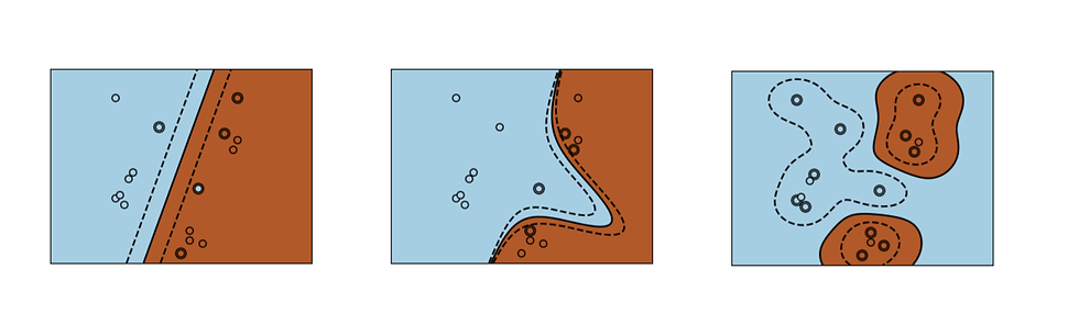
Image From: SciKit Learn. https://scikit-learn.org/stable/about.html#citing-scikit-learn

Linear Kernel

A linear kernel finds a decision boundary that is linear to separate the data into classes. Start by normalizing and splitting the data. Then train the model, predict the test data, and check the accuracy.

# Import required functions

from sklearn.datasets import make_classification

from sklearn.linear_model import LogisticRegression

from sklearn.model_selection import train_test_split

from sklearn.pipeline import make_pipeline

from sklearn.preprocessing import StandardScaler

# Split dataset into training set and test set

X_train, X_test, y_train, y_test = train_test_split(wine.data, wine.target, test_size=0.3,random_state=109) # 70% training and 30% test

# Make pipeline for normalizing data

pipe = make_pipeline(StandardScaler(), LogisticRegression())

pipe.fit(X_train, y_train) # apply scaling on training data

pipe.score(X_test, y_test) # apply scaling on testing data, without leaking training data.

0.9259259259259259

#Import svm model from sklearn import svm #Create a svm Classifier clf = svm.SVC(kernel='linear') # Linear Kernel #Train the model using the training sets clf.fit(X_train, y_train) #Predict the response for test dataset y_pred = clf.predict(X_test)

#Import scikit-learn metrics module for accuracy calculation

from sklearn import metrics

# Model Accuracy: how often is the classifier correct?

print("Accuracy:",metrics.accuracy_score(y_test, y_pred))

# Which classes are commonly misclassified?

print('Confusion Matrix')

print(metrics.confusion_matrix(y_test, y_pred, labels=None))

Accuracy: 0.9259259259259259

Confusion Matrix

[[21 0 0]

[ 3 15 1]

[ 0 0 14]]

It is not possible to plot a 13 dimensional graph, so to visualize the SVM decision boundary, we can train a new SVM model on just the first 2 features of the dataset and visualize the decision boundary in 2D.

from sklearn.svm import SVC

import numpy as np

import matplotlib.pyplot as plt

from sklearn import svm, datasets

# Select 2 features / variable for the 2D plot that we are going to create.

X = wine.data[:, :2] # we only take the first two features.

y = wine.target

def make_meshgrid(x, y, h=.02):

x_min, x_max = x.min() - 1, x.max() + 1

y_min, y_max = y.min() - 1, y.max() + 1

xx, yy = np.meshgrid(np.arange(x_min, x_max, h), np.arange(y_min, y_max, h))

return xx, yy

def plot_contours(ax, clf, xx, yy, **params):

Z = clf.predict(np.c_[xx.ravel(), yy.ravel()])

Z = Z.reshape(xx.shape)

out = ax.contourf(xx, yy, Z, **params)

return out

model = svm.SVC(kernel='linear')

clf = model.fit(X, y)

fig, ax = plt.subplots()

# Set-up grid for plotting.

X0, X1 = X[:, 0], X[:, 1]

xx, yy = make_meshgrid(X0, X1)

plot_contours(ax, clf, xx, yy, cmap=plt.cm.coolwarm, alpha=0.8)

ax.scatter(X0, X1, c=y, cmap=plt.cm.coolwarm, s=20, edgecolors='k')

ax.set_xlabel('Alcohol')

ax.set_ylabel('Malic Acid')

ax.set_title('Decision Surface of Linear SVM')

plt.show()