Applying Transformation with and without Spectral Clustering

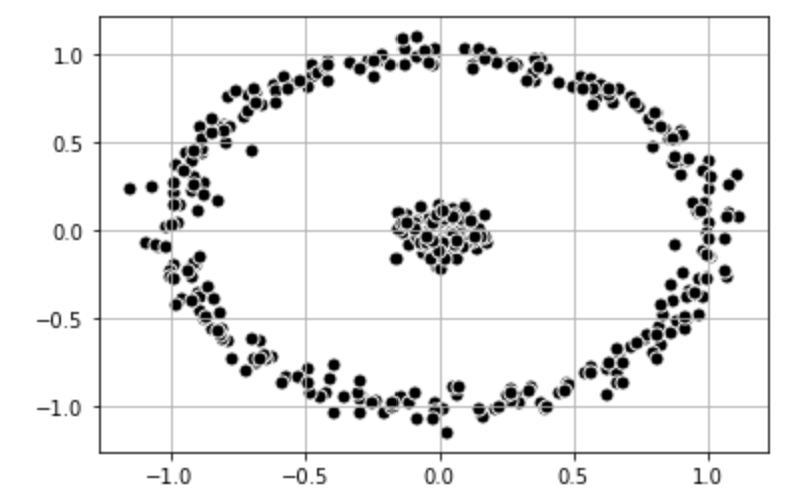
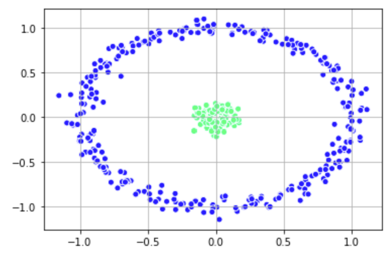
It is also possible to find other methods to change the dimensionality of the data. First, let's take a look at a dataset that consists of an inner circle and an outer ring. Spectral Clustering is able to classify the data.

import matplotlib.pyplot as plt

from sklearn.datasets import make_circles

# Generate data set

X_1, y_1 = make_circles(n_samples=(300, 100), shuffle=True, noise=0.05, factor=0.1, random_state=3)

# Plot data set

plt.scatter(

X_1[:, 0], X_1[:, 1],

c='black', marker='o',

edgecolor='white', s=50

)

plt.grid()

plt.show()

# Building the clustering model spectral_model_nn = SpectralClustering(n_clusters = 2, affinity ='nearest_neighbors') # Training the model and Storing the predicted cluster labels labels_nn = spectral_model_nn.fit_predict(X_1) plt.scatter(X_1[:, 0], X_1[:, 1], c = labels_nn, edgecolor='white', cmap =plt.cm.winter) plt.grid() plt.show()

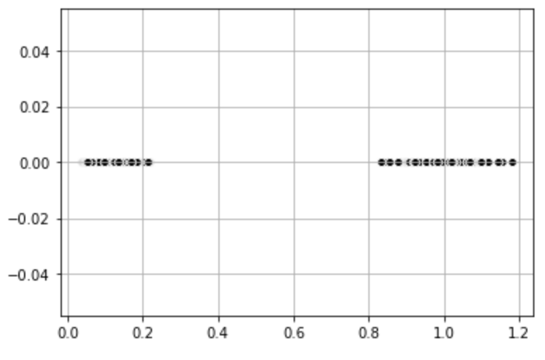
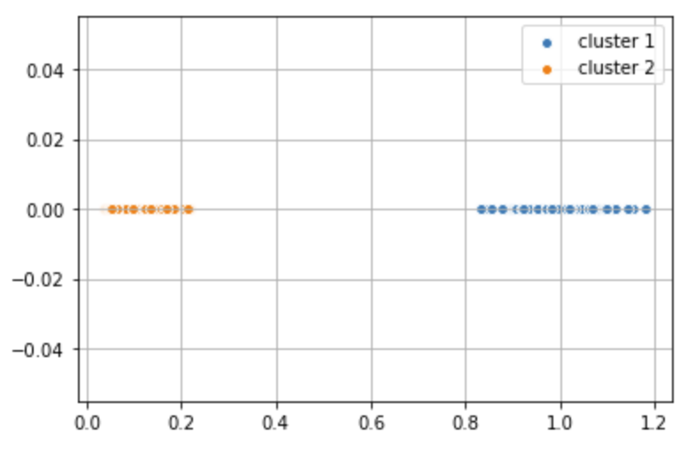
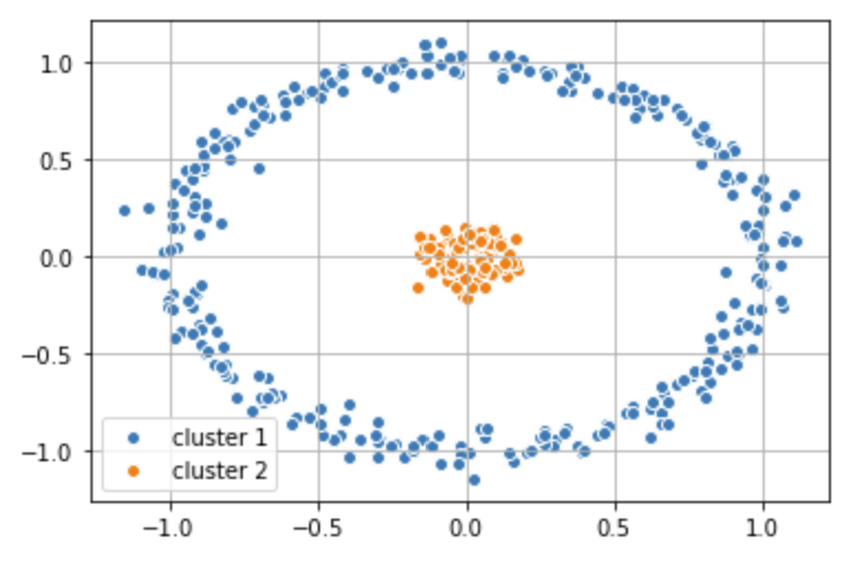
Alternatively, we can apply a transformation to the data set ourselves to reduce the dimensionality. For the dataset above, we can find the distance to the center (0,0) in this case. This transforms the dataset to one-dimensional space and the data becomes linearly separable. We can then apply K-Means to get the clusters.

import numpy as np

import copy

# Distance to 0,0

X_1_np = np.array(X_1) # points in dataset

dist = (X_1_np[:, 0] ** 2 + X_1_np[:, 1] ** 2) ** 0.5 # get distance to zero

dist_coord = np.array(list(zip(dist, np.zeros(dist.shape))))

# Plot

plt.scatter(dist_coord[:,0], dist_coord[:,1],

c = 'black', edgecolor='white', cmap =plt.cm.winter)

plt.grid()

plt.show()

from sklearn.cluster import KMeans

# K-Means with Visualization

km = KMeans(

n_clusters=2, init='random',

n_init=10, max_iter=300,

tol=1e-04, random_state=0

)

y_km = km.fit_predict(dist_coord) plt.scatter(dist_coord[y_km == 0,0], dist_coord[y_km == 0, 1], label = 'cluster 1', edgecolor='white', cmap =plt.cm.winter) plt.scatter(dist_coord[y_km == 1,0], dist_coord[y_km == 1, 1], label = 'cluster 2', edgecolor='white', cmap =plt.cm.winter) plt.legend(scatterpoints=1) plt.grid() plt.show()

# Apply labels determined by K-Means back to the origional data set

plt.scatter(X_1[y_km == 0,0], X_1[y_km == 0, 1],

label = 'cluster 1', edgecolor='white', cmap =plt.cm.winter)

plt.scatter(X_1[y_km == 1,0], X_1[y_km == 1, 1],

label = 'cluster 2', edgecolor='white', cmap =plt.cm.winter)

plt.legend(scatterpoints=1)

plt.grid()

plt.show()

TASK: Choose two features from the wine dataset which are appropriate for clustering and apply spectral clustering on the data based on those two features.

Don't forget to normalize the input data using a pipeline like we have done in previous notebooks. Check the SVM notebook for an example.