Import the dataset

# Import scikit-learn dataset library

from sklearn import datasets

# Load dataset

wine = datasets.load_wine()

# print the names of the 13 features print("Features: ", wine.feature_names) # print the label type of wine(class_0, class_1, class_2) print("Labels: ", wine.target_names)

Features: ['alcohol', 'malic_acid', 'ash', 'alcalinity_of_ash', 'magnesium', 'total_phenols', 'flavanoids', 'nonflavanoid_phenols', 'proanthocyanins', 'color_intensity', 'hue', 'od280/od315_of_diluted_wines', 'proline']

Labels: ['class_0' 'class_1' 'class_2']

# print data(feature)shape wine.data.shape

(178, 13)

Train the model

# Import train_test_split function from sklearn.model_selection import train_test_split # Split dataset into training set and test set X_train, X_test, y_train, y_test = train_test_split(wine.data, wine.target, test_size=0.3,random_state=109) # 70% training and 30% test

from sklearn.preprocessing import StandardScaler

scaler = StandardScaler()

# Fit only to the training data

scaler.fit(X_train)

# Now apply the transformations to the data:

X_train = scaler.transform(X_train)

X_test = scaler.transform(X_test)

from sklearn.neural_network import MLPClassifier

mlp = MLPClassifier(hidden_layer_sizes=(50,50,50), activation='relu', solver='adam', max_iter=200)

mlp.fit(X_train,y_train)

predict_train = mlp.predict(X_train)

predict_test = mlp.predict(X_test)

print(predict_test)

[0 0 1 2 0 1 0 0 1 0 1 1 2 2 0 1 1 0 0 1 2 1 0 2 0 0 1 2 0 1 2 1 1 0 1 2 0 2 2 0 2 0 0 0 0 2 2 0 1 1 2 1 0 2]

Evaluate model performance

To evaluate the performance of a neural network, it is possible to use similar metrics to those used before like checking the accuracy and printing a confusion matrix. Through SciKit Learn, it is also possible to get the precision, recall, and f1-score of each class.

Precision

• Precision: is the number of true positive results divided by the total predicted positive values

• The total predicted positive values is the sum of the number of true positive results and the false positive results

• For multiple classes, it is the number of correctly classified samples of that class divided by the total number of samples that the classifier assigned to that class

Recall

• Recall: is the number of true positive results divided by the total number of positive results

• The total positive results is the sum of the number of true positive results and the false negative results

• For multiple classes, it is the number of correctly classified samples of that class divided by the total number of samples that actually belong to that class

F-score

• F-score is equal to two times the precision times the recall divided by the precision plus the recall

mlp.score(X_test, y_test)

0.9629629629629629

# Performance on training dataset from sklearn.metrics import classification_report,confusion_matrix

# import required modules import numpy as np import matplotlib.pyplot as plt import seaborn as sns import pandas as pd class_names=[0,1,2] # name of classes fig, ax = plt.subplots() tick_marks = np.arange(len(class_names)) plt.xticks(tick_marks, class_names) plt.yticks(tick_marks, class_names)

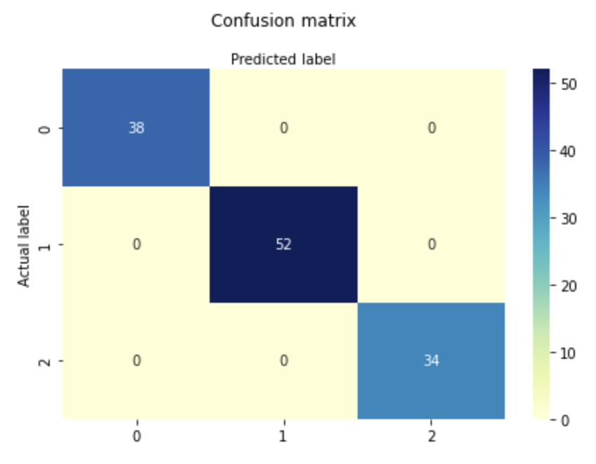
# create heatmap sns.heatmap(pd.DataFrame(confusion_matrix(y_train,predict_train)), annot=True, cmap="YlGnBu" ,fmt='g') ax.xaxis.set_label_position("top") plt.tight_layout() plt.title('Confusion matrix', y=1.1) plt.ylabel('Actual label') plt.xlabel('Predicted label') print(classification_report(y_train,predict_train))

precision recall f1-score support

0 1.00 1.00 1.00 38

1 1.00 1.00 1.00 52

2 1.00 1.00 1.00 34

accuracy 1.00 124

macro avg 1.00 1.00 1.00 124

weighted avg 1.00 1.00 1.00 124

# Performance on testing dataset

from sklearn.metrics import classification_report,confusion_matrix

# import required modules

import numpy as np

import matplotlib.pyplot as plt

import seaborn as sns

import pandas as pd

class_names=[0,1,2] # name of classes

fig, ax = plt.subplots()

tick_marks = np.arange(len(class_names))

plt.xticks(tick_marks, class_names)

plt.yticks(tick_marks, class_names)

# create heatmap

sns.heatmap(pd.DataFrame(confusion_matrix(y_test,predict_test)), annot=True, cmap="YlGnBu" ,fmt='g')

ax.xaxis.set_label_position("top")

plt.tight_layout()

plt.title('Confusion matrix', y=1.1)

plt.ylabel('Actual label')

plt.xlabel('Predicted label')

print(classification_report(y_test,predict_test))

precision recall f1-score support

0 0.95 1.00 0.98 21

1 1.00 0.89 0.94 19

2 0.93 1.00 0.97 14

accuracy 0.96 54

macro avg 0.96 0.96 0.96 54

weighted avg 0.97 0.96 0.96 54

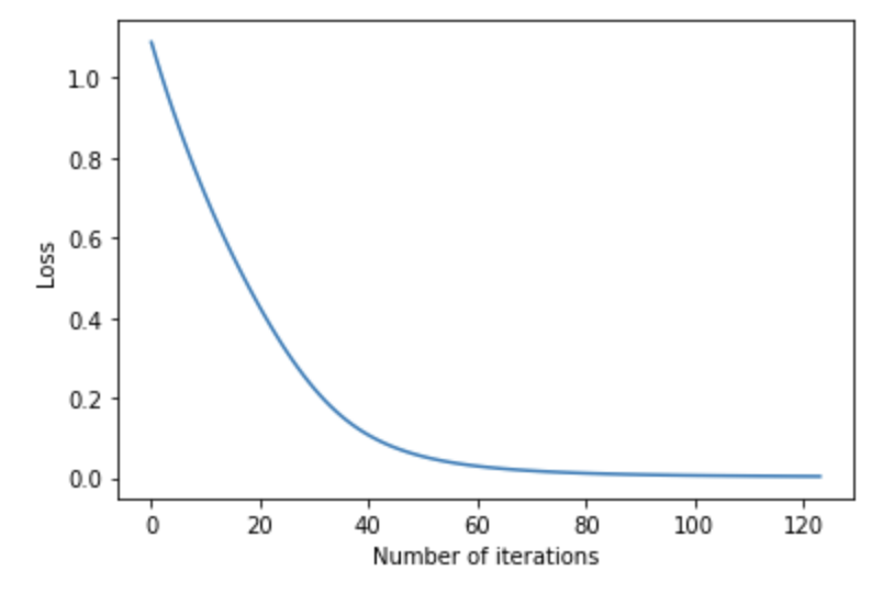
SciKit Learn also tracks the loss curve along the training iterations. By plotting the loss against the iterations, it is possible to visualize if the model is learning. If the loss curve decreases first quickly, and then more slowly like the one below, the neural network is learning. If the loss curve jumps between high and low values or starts by decreasing and then jumps between high and low values, there may be problems with the model (for example, maybe the learning rate is too high) or with the data set (for example, too many outliers or noise in your data set).

import matplotlib.pyplot as plt

fig, ax = plt.subplots(figsize=(6,4))

ax.plot(mlp.loss_curve_)

ax.set_xlabel('Number of iterations')

ax.set_ylabel('Loss')

plt.show()