Another way to see accuracy of training process

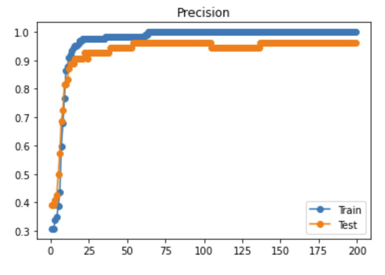
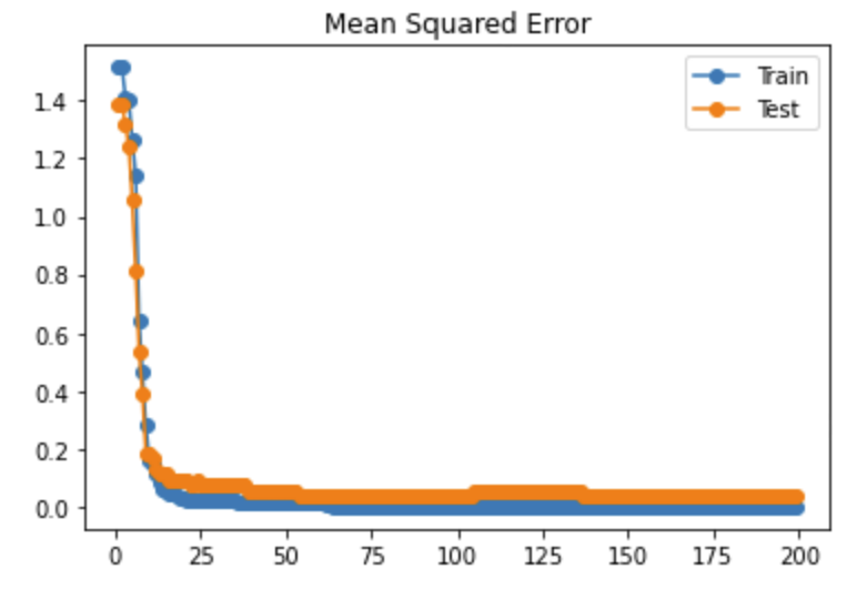
SciKit Learn does not track the accuracy of the training and testing data separately, but when you track these for each iteration and add them to a list it is possible to plot these two metrics at the end. When the curves are similar, it shows that the weights and biases used apply well to the training data and the test data. Additionally, you can track the mean squared error for each iteration and add them to a list to also plot the mean squared error of the train and test data against the training iteration.

from sklearn.metrics import accuracy_score, mean_squared_error

# define lists to collect scores

train_scores, test_scores = list(), list()

mse_train_scores, mse_test_scores = list(), list()

epochs = [i for i in range(1, 200)]

# evaluate for each iteration over 150 iteration

# configure the model

mlp2 = MLPClassifier(hidden_layer_sizes=(50,50,50), activation='relu', solver='adam', max_iter=200, batch_size="auto")

for epoch in epochs:

# fit model on the training dataset

mlp2 = mlp2.partial_fit(X_train, y_train, wine.target)

# evaluate on the train dataset

train_output = mlp2.predict(X_train)

train_acc = accuracy_score(y_train, train_output)

mse_train_acc = mean_squared_error(y_train, train_output)

mse_train_scores.append(mse_train_acc)

train_scores.append(train_acc)

# evaluate on the test dataset

test_output = mlp2.predict(X_test)

test_acc = accuracy_score(y_test, test_output)

mse_test_acc = mean_squared_error(y_test, test_output)

mse_test_scores.append(mse_test_acc)

test_scores.append(test_acc)

# summarize progress

print('>%d, train: %.3f, test: %.3f' % (epoch, train_acc, test_acc))

Output exceeds the size limit. Open the full output data in a text editor

>1, train: 0.306, test: 0.389

>2, train: 0.306, test: 0.389

>3, train: 0.339, test: 0.407

>4, train: 0.347, test: 0.426

>5, train: 0.387, test: 0.500

>6, train: 0.435, test: 0.574

>7, train: 0.597, test: 0.685

>8, train: 0.677, test: 0.722

>9, train: 0.766, test: 0.815

>10, train: 0.863, test: 0.815

>11, train: 0.879, test: 0.833

>12, train: 0.911, test: 0.870

>13, train: 0.919, test: 0.889

>14, train: 0.935, test: 0.889

>15, train: 0.944, test: 0.889

>16, train: 0.952, test: 0.907

>17, train: 0.952, test: 0.907

>18, train: 0.960, test: 0.907

>19, train: 0.968, test: 0.907

>20, train: 0.968, test: 0.907

>21, train: 0.976, test: 0.907

>22, train: 0.976, test: 0.926

>23, train: 0.976, test: 0.926

>24, train: 0.976, test: 0.907

>25, train: 0.976, test: 0.926

...

>196, train: 1.000, test: 0.963

>197, train: 1.000, test: 0.963

>198, train: 1.000, test: 0.963

>199, train: 1.000, test: 0.963

plt.plot(epochs, train_scores, '-o', label='Train') plt.plot(epochs, test_scores, '-o', label='Test') plt.title('Precision') plt.legend() plt.show()

plt.plot(epochs, mse_train_scores, '-o', label='Train')

plt.plot(epochs, mse_test_scores, '-o', label='Test')

plt.title('Mean Squared Error')

plt.legend()

plt.show()

TASK 1: Find a method or write a method yourself to do 5-fold cross validation with the training data.

TASK 2: Experiment with the neural network architecture. For example, change the depth or the width to improve the accuracy to be above 95%.