
Naive Bayes Classifiers (multi-label)
Introduction & Dataset
Naive Bayes classifiers for multiple labels work similar to naive Bayes classifiers for two classes. In this case, we will be looking 13 different features of wine: alcohol, malic acid, ash, alcalinity of ash, magnesium, total phenols, flavanoids, nonflavanoid phenols, proanthocyanins, color intensity, hue, od280/od315 of diluted wines, and proline. Based on these 13 features, the wine will be categorized into three classes: Class 0 (y1), Class 1 (y2), and Class 2 (y3). This time, the features are continuous, not discrete.
Again, the priors, or the probabilities of wine being assigned to a particular class, must be known. For the example below, the data is available for 178 wines. 59 wines were classified as Class 0 (y1) so the probability of the wine being assigned to Class 0 (P(y1)), is equal to 59/178. 71 wines were classified as Class 1 (y2) so the probability of the wine being assigned to Class 1 (P(y2)), is equal to 71/178. 48 wines were classified as Class 2 (y3) so the probability of the wine being assigned to Class 2 (P(y3)), is equal to 48/178.
Because the dataset uses continuous features, the likelihood is represented by the probability density function (p(X|yi) where i = 1, 2, 3).The process is similar to classifying into two classes except now look at the probability of three classes.
If P(y2|X) < P(y1|X) and P(y3|X) < P(y1|X), assign sample X to y1
If the probability of the wine being of Class 0 given the features is greater than the probability of the wine being of Class 1 and is greater than the probability of the wine being of Class 2, then the features are assigned to Class 0.
If P(y1|X) < P(y2|X) and P(y3|X) < P(y2|X), assign sample X to y2
If the probability of the wine being of Class 1 given the features is greater than the probability of the wine being of Class 0 and is greater than the probability of the wine being of Class 2, then the features are assigned to Class 1.
If P(y1|X) < P(y3|X) and P(y2|X) < P(y3|X), assign sample X to y3
If the probability of the wine being of Class 2 given the features is greater than the probability of the wine being of Class 0 and is greater than the probability of the wine being of Class 1, then the features are assigned to Class 2.

Figure 1: (Left) Likelihood represented by the probability density function (p(X|yi) where i = 1, 2, 3) (Center) Likelihood multiplied by class priors (Right) Obtain class posterior probabilities and determine the decision boundaries.
Let's take a look at implementing a naive Bayes Classifier with more than two classes with SciKit Learn.
Load the wine dataset and assign it to a variable. Print the name of the featues and labels to see the features and classes of the dataset.
# Import scikit-learn dataset library
from sklearn import datasets
from scipy.stats.kde import gaussian_kde
import numpy as np
import matplotlib.pyplot as plt
# Load dataset
wine = datasets.load_wine()
# print the names of the 13 features
print("Features: ", wine.feature_names)
# print the label type of wine(class_0, class_1, class_2)
print("Labels: ", wine.target_names)
Features: ['alcohol', 'malic_acid', 'ash', 'alcalinity_of_ash', 'magnesium', 'total_phenols', 'flavanoids', 'nonflavanoid_phenols', 'proanthocyanins', 'color_intensity', 'hue', 'od280/od315_of_diluted_wines', 'proline'] Labels: ['class_0' 'class_1' 'class_2']
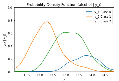
By running the code below, the likelihood of the feature alcohol given the three classes (0, 1, and 2) is graphed. The likelihood is represented by the probability mass function (p(X|y1)).
alcohol = wine.data[:, 0]
classes = wine.target
alcohol_class0 = [w[0] for w in zip(alcohol, classes) if w[1] == 0]
alcohol_class1 = [w[0] for w in zip(alcohol, classes) if w[1] == 1]
alcohol_class2 = [w[0] for w in zip(alcohol, classes) if w[1] == 2]
classes_all = ["Class 0", "Class 1", "Class 2"]
kde_0 = gaussian_kde(alcohol_class0)
dist_space_0 = np.linspace(0, 15, 250)
kde_1 = gaussian_kde(alcohol_class1)
dist_space_1 = np.linspace(0, 15, 250)
kde_2 = gaussian_kde(alcohol_class2)
dist_space_2 = np.linspace(0, 15, 250)
# plot the results
plt.title('Probability Density Function (alcohol | y_i)')
plt.ylim((0, 1))plt.xlim((np.amin(alcohol), np.amax(alcohol)))
plt.xlabel('x') plt.ylabel('p(x | y_i)')
plt.plot(dist_space_0, kde_0(dist_space_0), label='y_1 Class 0')
plt.plot(dist_space_1, kde_1(dist_space_1), label='y_2 Class 1')
plt.plot(dist_space_2, kde_2(dist_space_2), label='y_3 Class 2')
plt.legend()
plt.show()
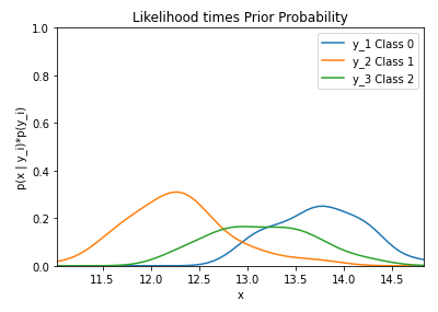
By running the code below, the likelihood of the feature alcohol given the three classes (0, 1, and 2) multiplied by the priors of each class is graphed.
alcohol = wine.data[:, 0]
classes = wine.target
alcohol_class0 = [w[0] for w in zip(alcohol, classes) if w[1] == 0]
alcohol_class1 = [w[0] for w in zip(alcohol, classes) if w[1] == 1]
alcohol_class2 = [w[0] for w in zip(alcohol, classes) if w[1] == 2]
classes_all = ["Class 0", "Class 1", "Class 2"]
kde_0 = gaussian_kde(alcohol_class0)
dist_space_0 = np.linspace(0, 15, 250)
kde_1 = gaussian_kde(alcohol_class1)
dist_space_1 = np.linspace(0, 15, 250)
kde_2 = gaussian_kde(alcohol_class2)
dist_space_2 = np.linspace(0, 15, 250)
# plot the results
plt.title('Likelihood * Class Priors')
plt.ylim((0, 1))
plt.xlim((np.amin(alcohol), np.amax(alcohol)))
plt.xlabel('x')
plt.ylabel('p(x | y_i)*p(y_i)')
plt.plot(dist_space_0, kde_0(dist_space_0) * (len(alcohol_class0) / len(alcohol)), label='y_1 Class 0')
plt.plot(dist_space_1, kde_1(dist_space_1) * (len(alcohol_class1) / len(alcohol)), label='y_2 Class 1')
plt.plot(dist_space_2, kde_2(dist_space_2) * (len(alcohol_class2) / len(alcohol)), label='y_3 Class 2')
plt.legend()
plt.show()
We can print a number of pieces of information to understand some of the characteristics of the dataset.