
Multinomial Logistic Regression | Notebook
Load the dataset and print some the information about the dataset.
# Import scikit-learn dataset library
from sklearn import datasets
# Load dataset
wine = datasets.load_wine()
# print the names of the features
print(wine.feature_names)
['alcohol', 'malic_acid', 'ash', 'alcalinity_of_ash', 'magnesium', 'total_phenols', 'flavanoids', 'nonflavanoid_phenols', 'proanthocyanins', 'color_intensity', 'hue', 'od280/od315_of_diluted_wines', 'proline']
# print the label species(class_0, class_1, class_2) print(wine.target_names)
['class_0' 'class_1' 'class_2']
# print the wine data (top 5 records)
print(wine.data[0:5])
[[1.423e+01 1.710e+00 2.430e+00 1.560e+01 1.270e+02 2.800e+00 3.060e+00
2.800e-01 2.290e+00 5.640e+00 1.040e+00 3.920e+00 1.065e+03] [1.320e+01 1.780e+00 2.140e+00 1.120e+01 1.000e+02 2.650e+00 2.760e+00
2.600e-01 1.280e+00 4.380e+00 1.050e+00 3.400e+00 1.050e+03] [1.316e+01 2.360e+00 2.670e+00 1.860e+01 1.010e+02 2.800e+00 3.240e+00
3.000e-01 2.810e+00 5.680e+00 1.030e+00 3.170e+00 1.185e+03] [1.437e+01 1.950e+00 2.500e+00 1.680e+01 1.130e+02 3.850e+00 3.490e+00
2.400e-01 2.180e+00 7.800e+00 8.600e-01 3.450e+00 1.480e+03] [1.324e+01 2.590e+00 2.870e+00 2.100e+01 1.180e+02 2.800e+00 2.690e+00
3.900e-01 1.820e+00 4.320e+00 1.040e+00 2.930e+00 7.350e+02]]
# print the wine labels (0:Class_0, 1:Class_1, 2:Class_3) print(wine.target)
[0 0 0 0 0 0 0 0 0 0 0 0 0 0 0 0 0 0 0 0 0 0 0 0 0 0 0 0 0 0 0 0 0 0 0 0 0 0 0 0 0 0 0 0 0 0 0 0 0 0 0 0 0 0 0 0 0 0 0 1 1 1 1 1 1 1 1 1 1 1 1 1 1 1 1 1 1 1 1 1 1 1 1 1 1 1 1 1 1 1 1 1 1 1 1 1 1 1 1 1 1 1 1 1 1 1 1 1 1 1 1 1 1 1 1 1 1 1 1 1 1 1 1 1 1 1 1 1 1 1 2 2 2 2 2 2 2 2 2 2 2 2 2 2 2 2 2 2 2 2 2 2 2 2 2 2 2 2 2 2 2 2 2 2 2 2 2 2 2 2 2 2 2 2 2 2 2 2]
# print data(feature)shape
print(wine.data.shape)
(178, 13)
# print target(or label)shape
print(wine.target.shape)
(178,)
Train model with one feature
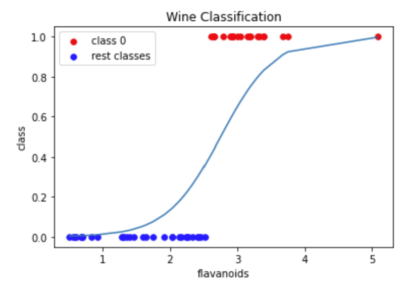
First, we will train the classifier and predict the classes of the data using only one feature so we can visualize the probability curve for the data.
# import the class
from sklearn.model_selection import train_test_split
from sklearn.linear_model import LogisticRegression
from sklearn import preprocessing
from sklearn import metrics
#feature 6, flavanoids, results in highest accuracy (78%), feature 0, alcohol, also has fairly high accuracy (74%)
feature = 6
# Split dataset into training set and test set
X_train, X_test, y_train, y_test = train_test_split(wine.data[:, feature].reshape(-1, 1), wine.target, test_size=0.3) # 70% training and 30% test
# instantiate the model (using the default parameters)
logreg = LogisticRegression(multi_class="multinomial", max_iter=10000)
# fit the model with data
logreg.fit(X_train, y_train)
y_pred = logreg.predict(X_test)
print("Accuracy:",metrics.accuracy_score(y_test, y_pred))
cnf_matrix = metrics.confusion_matrix(y_test, y_pred)
print("Confusion Matrix:", cnf_matrix)
Accuracy: 0.6851851851851852
Confusion Matrix: [[13 4 0]
[ 9 15 4]
[ 0 0 9]]
import numpy as np
import matplotlib.pyplot as plt
import math
# plot class 0 versus the rest to show probability curve
# update list so 0 is class 0 and 1 is "rest"
y_pred_class0 = [1 for x in y_pred if x == 0]
y_pred_classrest = [0 for x in y_pred if x > 0]
X_class0 = [X_test[i, 0] for i, x in enumerate(y_pred) if x == 0]
X_classrest = [X_test[i,0] for i, x in enumerate(y_pred) if x != 0]
X_value = X_test[:,0]
X_value.sort()
sigmoid = [1/(1+math.exp(2.5*-(x-2.75))) for x in X_value]
plt.scatter(X_class0, y_pred_class0, s=30, c='r', label='class 0')
plt.scatter(X_classrest, y_pred_classrest, s=30, c='b', label='rest classes')
plt.plot(X_value,sigmoid)
plt.title('Wine Classification')
plt.xlabel('flavanoids')
plt.ylabel('class')
plt.legend()
plt.show()
Train Model with all Features
Now, train a classifier and predict the classes of the data.
Split the data into a train and test set based on a 70/30 split.
# Import train_test_split function
from sklearn.model_selection import train_test_split
# Split dataset into training set and test set
X_train, X_test, y_train, y_test = train_test_split(wine.data, wine.target, test_size=0.3) # 70% training and 30% test
# import the class
from sklearn.linear_model import LogisticRegression
from sklearn import preprocessing
# instantiate the model (using the default parameters)
logreg = LogisticRegression(multi_class="multinomial", max_iter=10000)
# fit the model with data
logreg.fit(X_train, y_train)
y_pred = logreg.predict(X_test)
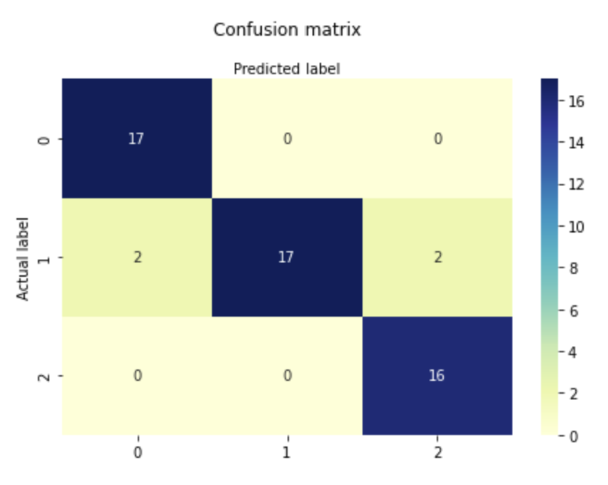
Check the performance of the model by printing the confusion matrix and also plotting the confusion matrix.
# import the metrics class
from sklearn import metrics
print("Accuracy:",metrics.accuracy_score(y_test, y_pred))
cnf_matrix = metrics.confusion_matrix(y_test, y_pred)
print("Confusion Matrix:", cnf_matrix)
Accuracy: 0.9259259259259259
Confusion Matrix: [[17 0 0]
[ 2 17 2]
[ 0 0 16]]
# import required modules
import numpy as np
import matplotlib.pyplot as plt
import seaborn as sns
import pandas as pd
class_names=[0,1,2] # name of classes
fig, ax = plt.subplots()
tick_marks = np.arange(len(class_names))
plt.xticks(tick_marks, class_names)
plt.yticks(tick_marks, class_names)
# create heatmap
sns.heatmap(pd.DataFrame(cnf_matrix), annot=True, cmap="YlGnBu" ,fmt='g')
ax.xaxis.set_label_position("top")
plt.tight_layout()
plt.title('Confusion matrix', y=1.1)
plt.ylabel('Actual label')
plt.xlabel('Predicted label')
Text(0.5, 257.44, 'Predicted label')
Evaluate model performance
To evaluate the performance of multinomial logistic regression, it is possible to use similar metrics to those used before, like checking the accuracy and printing a confusion matrix. Through SciKit Learn, it is also possible to get the precision, recall, and f1-score of each class.
Precision
Precision: is the number of true positive results divided by the total predicted positive values
The total predicted positive values is the sum of the number of true positive results and the false positive results
For multiple classes, it is the number of correctly classified samples of that class divided by the total number of samples that the classifier assigned to that class
Recall
Recall: is the number of true positive results divided by the total number of positive results
The total positive results is the sum of the number of true positive results and the false negative results
For multiple classes, it is the number of correctly classified samples of that class divided by the total number of samples that actually belong to that class
F-score
F-score is equal to two times the precision times the recall divided by the precision plus the recall
F-score = 2 * (precision * recall) / (precision + recall)