# Import scikit-learn dataset library

from sklearn import datasets

# Load dataset

wine = datasets.load_wine()

As we discussed previously, it can be helpful to print certain characteristics of the dataset.

# print the names of the features

print(wine.feature_names)

['alcohol', 'malic_acid', 'ash', 'alcalinity_of_ash', 'magnesium', 'total_phenols', 'flavanoids', 'nonflavanoid_phenols', 'proanthocyanins', 'color_intensity', 'hue', 'od280/od315_of_diluted_wines', 'proline']

# print the label species (class_0, class_1, class_2)

print(wine.target_names)

['class_0' 'class_1' 'class_2']

# print data(feature)shape

print(wine.data.shape)

(178, 13)

# print the wine data (top 5 records)

print(wine.data[0:5])

[[1.423e+01 1.710e+00 2.430e+00 1.560e+01 1.270e+02 2.800e+00 3.060e+00

2.800e-01 2.290e+00 5.640e+00 1.040e+00 3.920e+00 1.065e+03]

[1.320e+01 1.780e+00 2.140e+00 1.120e+01 1.000e+02 2.650e+00 2.760e+00

2.600e-01 1.280e+00 4.380e+00 1.050e+00 3.400e+00 1.050e+03]

[1.316e+01 2.360e+00 2.670e+00 1.860e+01 1.010e+02 2.800e+00 3.240e+00

3.000e-01 2.810e+00 5.680e+00 1.030e+00 3.170e+00 1.185e+03]

[1.437e+01 1.950e+00 2.500e+00 1.680e+01 1.130e+02 3.850e+00 3.490e+00

2.400e-01 2.180e+00 7.800e+00 8.600e-01 3.450e+00 1.480e+03]

[1.324e+01 2.590e+00 2.870e+00 2.100e+01 1.180e+02 2.800e+00 2.690e+00

3.900e-01 1.820e+00 4.320e+00 1.040e+00 2.930e+00 7.350e+02]]

# print target(or label)

shapeprint(wine.target.shape)

(178,)

# print the wine labels (0:Class_0, 1:Class_1, 2:Class_3)

print(wine.target)

[0 0 0 0 0 0 0 0 0 0 0 0 0 0 0 0 0 0 0 0 0 0 0 0 0 0 0 0 0 0 0 0 0 0 0 0 0 0 0 0 0 0 0 0 0 0 0 0 0 0 0 0 0 0 0 0 0 0 0 1 1 1 1 1 1 1 1 1 1 1 1 1 1 1 1 1 1 1 1 1 1 1 1 1 1 1 1 1 1 1 1 1 1 1 1 1 1 1 1 1 1 1 1 1 1 1 1 1 1 1 1 1 1 1 1 1 1 1 1 1 1 1 1 1 1 1 1 1 1 1 2 2 2 2 2 2 2 2 2 2 2 2 2 2 2 2 2 2 2 2 2 2 2 2 2 2 2 2 2 2 2 2 2 2 2 2 2 2 2 2 2 2 2 2 2 2 2 2]

Features and Classification

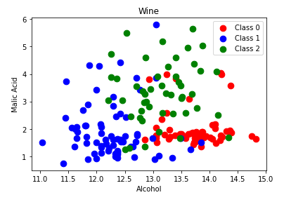
Remember that K-Nearest Neighbors classification graphs the existing records and associated labels. When an unknown datapoint needs to be classified, the distance to all other datapoints is measured. Then, the k nearest neighbors are retrieved and based on which label is most common within this group, a predicted label is determined. Plot two of the features of the dataset: alcohol and malic_acid. We can see how even with only two of the 13 features, the values given a specific class are located near each other.

import numpy as np

import matplotlib.pyplot as plt

alcohol = wine.data[:, 0]

malic_acid = wine.data[:,1]

classes = wine.target

features = list(zip(alcohol, malic_acid))

# plot the records here

class_0 = np.array([w[0] for w in zip(features, classes) if w[1] == 0])

class_1 = np.array([w[0] for w in zip(features, classes) if w[1] == 1])

class_2 = np.array([w[0] for w in zip(features, classes) if w[1] == 2])

plt.scatter(class_0[:, 0], class_0[:, 1], s=75, c='r', label = "Class 0")

plt.scatter(class_1[:, 0], class_1[:, 1], s=75, c='b', label = "Class 1")

plt.scatter(class_2[:, 0], class_2[:, 1], s=75, c='g', label = "Class 2")

plt.title('Wine')

plt.xlabel('Alcohol')

plt.ylabel('Malic Acid')

plt.legend()

plt.show()

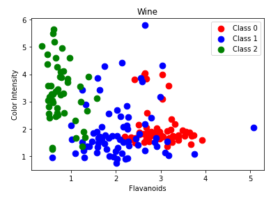
Also plot flavanoids and color_intensity.

import numpy as np

import matplotlib.pyplot as plt

flavanoids = wine.data[:, 6]

color_intensity = wine.data[:,9]

classes = wine.target

features = list(zip(flavanoids, malic_acid))

# plot the records here

class_0 = np.array([w[0] for w in zip(features, classes) if w[1] == 0])

class_1 = np.array([w[0] for w in zip(features, classes) if w[1] == 1])

class_2 = np.array([w[0] for w in zip(features, classes) if w[1] == 2])

plt.scatter(class_0[:, 0], class_0[:, 1], s=75, c='r', label = "Class 0")

plt.scatter(class_1[:, 0], class_1[:, 1], s=75, c='b', label = "Class 1")

plt.scatter(class_2[:, 0], class_2[:, 1], s=75, c='g', label = "Class 2")

plt.title('Wine')

plt.xlabel('Flavanoids')

plt.ylabel('Color Intensity')

plt.legend()

plt.show()

Train a classifier using a 70:30 train test split and print the accuracy.

# Import required functions

from sklearn.datasets

import make_classification

from sklearn.linear_model import LogisticRegression

from sklearn.model_selection import train_test_split

from sklearn.pipeline import make_pipeline

from sklearn.preprocessing import StandardScaler

# Split dataset into training set and test set8

X_train, X_test, y_train, y_test = train_test_split(wine.data, wine.target, test_size=0.3) # 70% training and 30% test

# Make pipeline for normalizing data

pipe = make_pipeline(StandardScaler(), LogisticRegression())

pipe.fit(X_train, y_train)  

# apply scaling on training data

pipe.score(X_test, y_test)  # apply scaling on testing data, without leaking training data.

0.9629629629629629

The k value is a parameter when generating the model. It is necessary to test a number of options for k because having a small value may increase the classifier's sensitivity to noise and having large value may lead to datapoints from other classes being included and impacting the accuracy.

# Import knearest neighbors Classifier model

from sklearn.neighbors import KNeighborsClassifier

# Create KNN Classifier

knn = KNeighborsClassifier(n_neighbors=5)

# Train the model using the training sets

knn.fit(X_train, y_train)

# Predict the response for test dataset

y_pred = knn.predict(X_test)print(y_pred)

[1 2 0 1 2 2 0 2 2 0 1 0 1 2 0 0 1 2 1 2 1 1 0 0 0 0 0 1 2 0 1 1 0 2 2 1 2 2 2 2 1 2 1 0 0 1 0 1 2 0 0 2 0 0]

# Import scikit-learn metrics module for accuracy calculation

from sklearn import metrics

# Model Accuracy, how often is the classifier correct?

print("Accuracy:",metrics.accuracy_score(y_test, y_pred))

# Import scikit-learn metrics module for confusion matrix

from sklearn import metrics

# Which classes are commonly misclassified?

print('Confusion Matrix')print(metrics.confusion_matrix(y_test, y_pred, labels=[0, 1, 2]))

Accuracy: 0.6851851851851852

Confusion Matrix [[16 0 1]

[ 4 14 10]

[ 0 2 7]]

As discussed, changing the k value changes the accuracy of the predictions. When K is too large, the classifier is less accurate.

# Import knearest neighbors Classifier model

from sklearn.neighbors import KNeighborsClassifier

# Create KNN Classifier

knn = KNeighborsClassifier(n_neighbors=12)

# Train the model using the training sets

knn.fit(X_train, y_train)

# Predict the response for test dataset

y_pred = knn.predict(X_test)

# Import scikit-learn metrics module for accuracy calculation

from sklearn import metrics

# Model Accuracy, how often is the classifier correct?

print("Accuracy:",metrics.accuracy_score(y_test, y_pred))

# Import scikit-learn metrics module for confusion matrix

from sklearn import metrics

# Which classes are commonly misclassified?

print('Confusion Matrix')

print(metrics.confusion_matrix(y_test, y_pred, labels=[0, 1, 2]))

Accuracy: 0.6851851851851852

Confusion Matrix [[16 0 1]

[2 14 12]

[ 1 1 7]]

TASK: Now that you know how to train a classifier and check the accuracy, try plotting the k value against the accuracy of the trained model.