# Load libraries

from sklearn.tree import DecisionTreeClassifier # Import Decision Tree Classifier

from sklearn.model_selection import train_test_split # Import train_test_split function

from sklearn import metrics # Import scikit-learn metrics module for accuracy calculation

# Import scikit-learn dataset library

from sklearn import datasets

# Load dataset

wine = datasets.load_wine()

It can be helpful to print certain characteristics of the dataset.

# print the names of the features

print(wine.feature_names)

['alcohol', 'malic_acid', 'ash', 'alcalinity_of_ash', 'magnesium', 'total_phenols', 'flavanoids', 'nonflavanoid_phenols', 'proanthocyanins', 'color_intensity', 'hue', 'od280/od315_of_diluted_wines', 'proline']

# print the label species(class_0, class_1, class_2)

print(wine.target_names)

['class_0' 'class_1' 'class_2']

Train a classifier using a 70/30 train test split and print the accuracy.

# Split dataset into training set and test set

X_train, X_test, y_train, y_test = train_test_split(wine.data, wine.target, test_size=0.3, random_state=1) # 70% training and 30% test

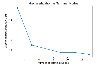
As discussed, it is possible to set the max_depth parameter allows control over the size of the tree to prevent overfitting. You can see the impact of overfitting by plotting the relative misclassification cost against the number of terminal nodes. The misclassification rate is calculated by taking the number of incorrect predictions and dividing these by the total number of predictions. The plot below shows that 9 terminal nodes is optimal because it allows for a low misclassification rate but the tree isn't too large for overfitting to be a problem.

# change this to max depth

from matplotlib import pyplot as plt

terminal_nodes = []

accuracy = []

for i in range(1, 6):   

# Create Decision Tree classifer object   

clf = DecisionTreeClassifier(max_depth=i)   

# Train Decision Tree Classifer   

clf = clf.fit(X_train,y_train)   

# Predict the response for test dataset append accuracy for plotting   

y_pred = clf.predict(X_test)   

terminal_nodes.append(clf.tree_.node_count)   

accuracy.append(1 - metrics.accuracy_score(y_test, y_pred))  

plt.plot(terminal_nodes, accuracy, '-o')

plt.title('Misclassification vs Terminal Nodes')

plt.xlabel('Number of Terminal Nodes')

plt.ylabel('Relative Misclassification Cost')

plt.show()

TASK 1: When training the model, the hyperparameter for the SciKit function is the maximum depth, not the number of terminal nodes. Now plot the Relative Misclassification Cost against the Maximum Depth to decide which max_depth value to use for the classifier.

TASK 2: The classifier below is trained with a max_depth value of 2. Based on the plot above, what value is more accurate? Update the max_depth value below.

# Create Decision Tree classifer object

clf = DecisionTreeClassifier(max_depth = 2)

# Train Decision Tree Classifer

clf = clf.fit(X_train,y_train)

# Predict the response for test dataset

y_pred = clf.predict(X_test)

print(y_pred)

[2 1 0 1 0 2 1 0 2 1 0 1 1 0 1 1 1 0 1 0 0 1 1 0 0 2 0 0 0 2 1 1 1 0 1 1 1 1 1 0 0 2 2 1 0 0 1 0 0 0 1 2 2 0]

# Number of Terminal Nodes

print("Terminal Node Count:", clf.tree_.node_count)

# Model Accuracy, how often is the classifier correct?

print("Accuracy:",metrics.accuracy_score(y_test, y_pred))

# Which classes are commonly misclassified?

print('Confusion Matrix')

print(metrics.confusion_matrix(y_test, y_pred, labels=None))

Terminal Node Count: 5

Accuracy: 0.8518518518518519

Confusion Matrix

[[21 2 0]

[ 1 17 1]

[ 0 4 8]]

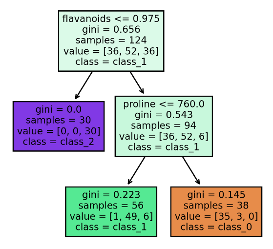
The plot_tree function allows us to plot a visualization of the decision tree generated by the trained classifier. The decision tree stopped splitting after a depth of 2 has been reached. When no maximum depth is set, the tree stops splitting into descendant nodes when the Gini impurity measure is 0. The challenge of not setting a depth is that overfitting can occur.

import matplotlib.pyplot as plt

from sklearn import tree

# Setting dpi = 300 to make image clearer than default

fig, axes = plt.subplots(nrows = 1,ncols = 1,figsize = (4,4), dpi=300)

tree.plot_tree(clf,

          feature_names = wine.feature_names,

      class_names=wine.target_names, 

     filled = True);